GVEC
a flexible 3D MHD equilibrium solver
Robert Babin
Max Planck Institute for Plasma Physics, NMPP
Outline
\[
\newcommand{\deriv}{\mathrm{d}}
\newcommand{\pqdx}[2]{\frac{\partial #1}{\partial #2}}
\newcommand{\dqdx}[2]{\frac{\deriv #1}{\deriv #2}}
\newcommand{\pqdxx}[2]{\frac{\partial^2 #1}{\partial {#2}^2}}
\newcommand{\dqdxx}[2]{\frac{\deriv^2 #1}{\deriv {#2}^2}}
\newcommand{\pqdxy}[3]{\frac{\partial^2 #1}{\partial #2 \partial #3}}
\newcommand{\grad}{\mathbf{\nabla}}
\newcommand{\vec}[1]{\mathbf{#1}}
\]
- Theoretical Background
- Tokamak
- Stellarator
- Postprocessing
- Flexible Coordinate Frame
- Questions & Discussion
Galerkin Variational Equilibrium Code
Goal: compute 3D ideal magnetohydrodynamic equilibria
- for toroidal magnetic confinement fusion plasmas \[
\begin{align}
\mathbf{J} \times \mathbf{B} &= \nabla p \\
\nabla \times \mathbf{B} &= \mu_0 \mathbf{J} \\
\nabla \cdot \mathbf{B} &= 0
\end{align}
\]
Minimize MHD energy \[ W = \int_\Omega \frac{|\mathbf{B}|^2}{2\mu_0} + \frac{p}{\gamma - 1} \, dV \]
Inspired by VMEC & DESC
Solve for the geometry of the magnetic field
- assume existence of nested flux surfaces
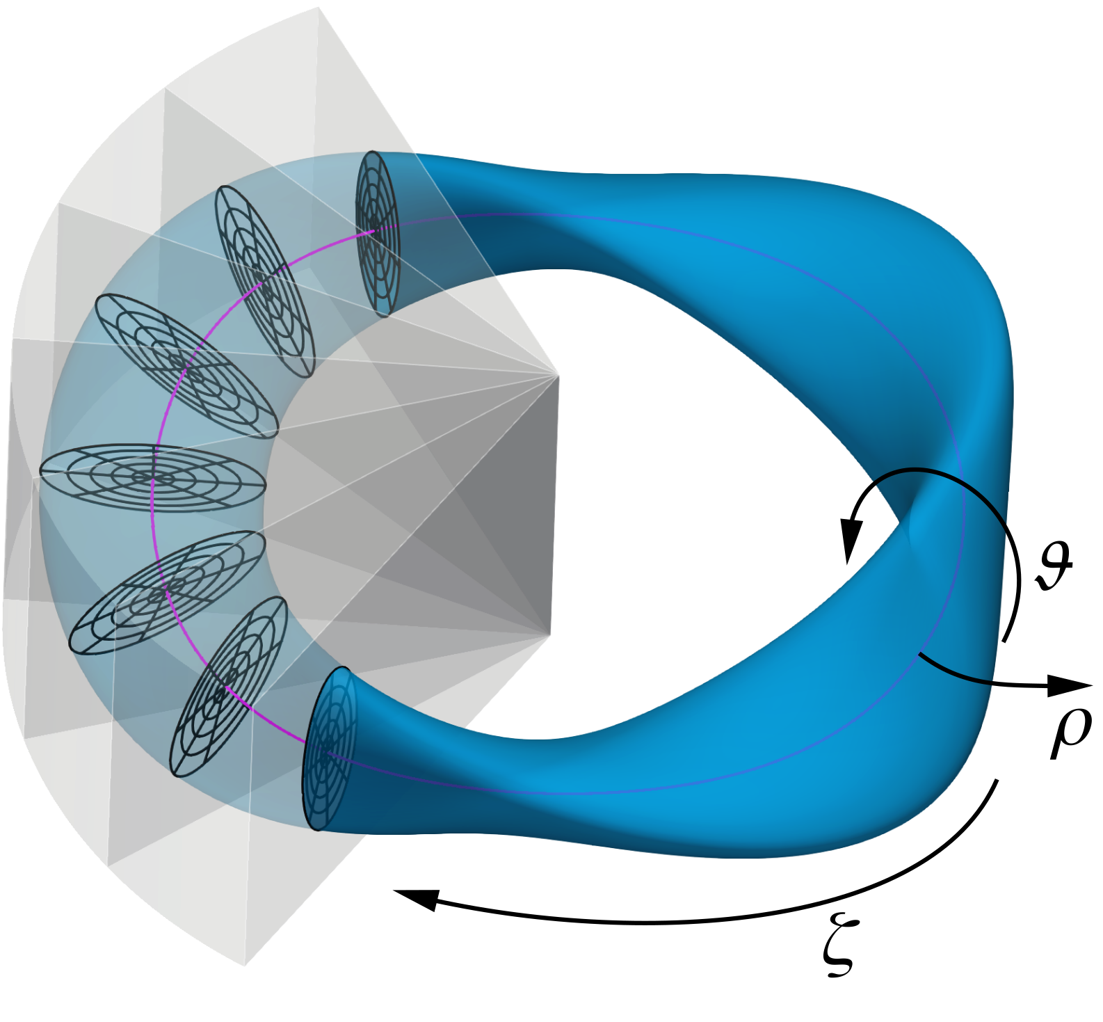
- inverse representation \(\mathbf{x}(\rho, \vartheta, \zeta)\)
- using flux-aligned coordinates \(\mathbf{B} = \nabla \Phi(\rho) \times \nabla (\vartheta + \lambda(\rho, \vartheta, \zeta)) - \nabla \chi(\rho) \times \nabla \zeta\)
- initial condition / background equilibrium for higher fidelity codes
Galerkin Variational Equilibrium Code
- Flexible coordinate frame – not restricted to cylindrical coordinates
- use any toroidal coordinate system: \((\rho,\vartheta,\zeta) \mapsto (q^1,q^2,\zeta) \mapsto (x,y,z)\)
- e.g. cylindrical coordinates: \(q^1 := R, q^2 := Z, \zeta := \varphi\)
- alternative: G-Frame – curve following coordinates
- Discretization: solve for \(X^1(\rho,\vartheta,\zeta), X^2(\rho,\vartheta,\zeta), \lambda(\rho,\vartheta,\zeta)\)
- B-Splines radially
- Fourier series poloidally & toroidally
- Smoothness constraint at the magnetic axis
- Enforce field periodicity & stellarator symmetry
- Developed at Max Planck Institute for Plasma Physics (Garching, Germany)
- Contributors: Florian Hindenlang, Omar Maj, Robert Babin, Robert Köberl, Dean Muir, Tiago Tamissa Ribeiro
- Open Source: gitlab.mpcdf.mpg.de/gvec-group/gvec
- Cite:
DOI:10.5281/zenodo.15026780 / JOSS paper under review
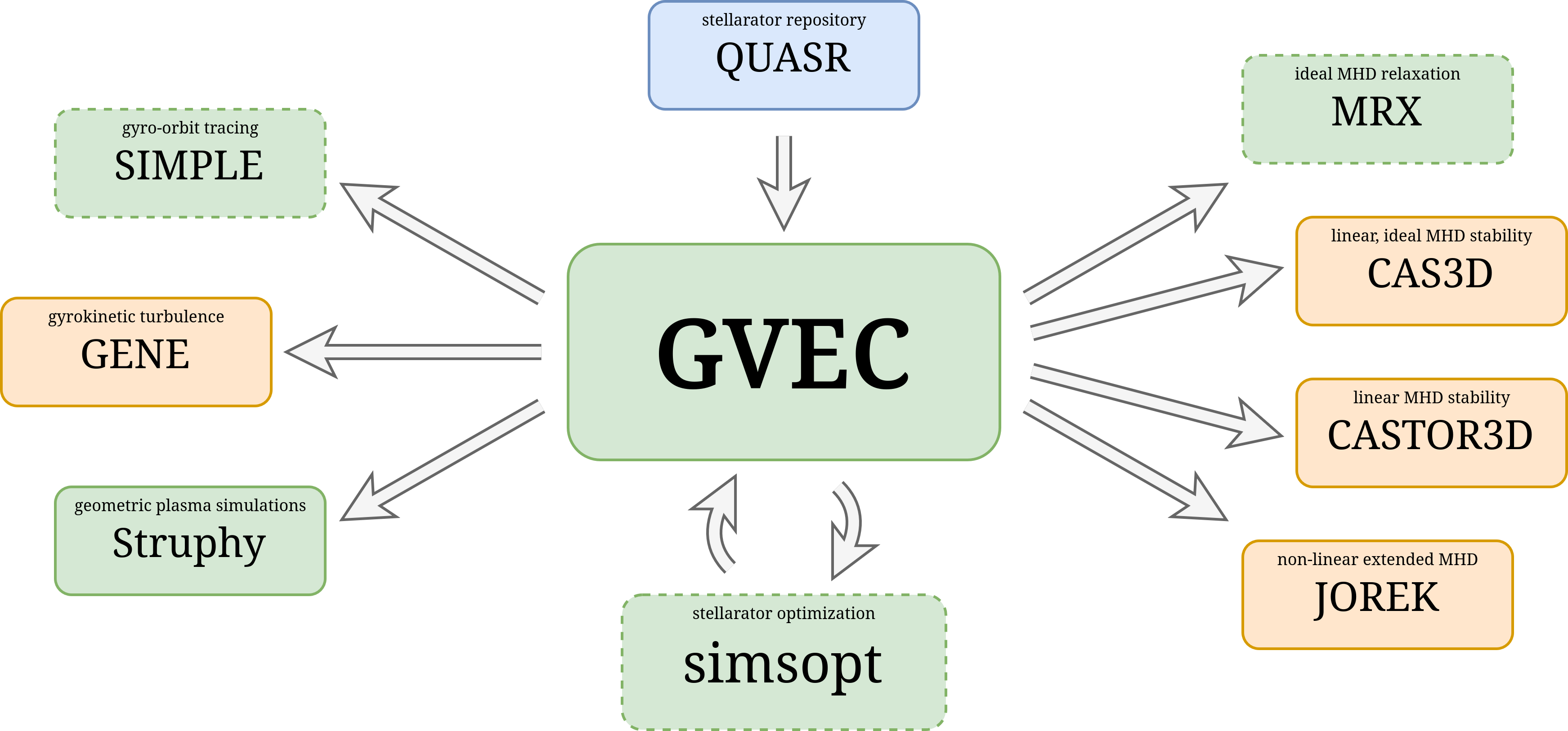
Interfaces
![]()
- green: open source software
- blue: public database
- orange: closed source software
- dashed: interface under development
Software Design Principles / Goals
- good & robust numerics
- performant implementation in Modern Fortran
- parallelization with OpenMP & MPI
- intuitive & simple interface through python (+ installation)
- interface API for postprocessing of equilibrium solutions
- gradual improvements rather than complete rewrite
- testing & documentation
- open source
Setup
- compiles GVEC on your machine (using
CMake & scikit-build-core)
- installs
gvec binary, pygvec scripts & gvec python package
- requires some system libraries (BLAS, netCDF, …)
- details / problems: gvec.readthedocs.io/install
import os
os.environ["OMP_NUM_THREADS"] = "2"
import gvec
print(gvec.__version__)
Computing an Equilibrium: Tokamak
For a fixed-boundary ideal MHD equilibrium, we need to specify:
- the physics parameters
- the boundary shape
- numerical parameters
Tokamak: Physics Parameters
- toroidal magnetic flux: \(\Phi(\rho^2) = \Phi_\text{edge} \rho^2\)
- rotational transform profile: \(\iota(\rho^2)\)
- pressure profile: \(p(\rho^2)\)
params = {
"PhiEdge": 1.0,
"iota": {
"type": "polynomial",
"coefs": [0.625, 0.35],
},
"pres": {
"type": "interpolation",
"rho2": [0.0, 0.25, 0.5, 0.75, 1.0],
"vals": [1.0, 0.75, 0.5, 0.25, 0.0],
"scale": 1000.0,
}
}
Tokamak: Coordinate Frame
Choose cylindrical coordinates:
\[
(x,y,z) := (R\cos\zeta, -R\sin\zeta, Z)\\
R = X^1(\rho,\vartheta,\zeta) \\
Z = X^2(\rho,\vartheta,\zeta)
\]
params["which_hmap"] = 1 # cylindrical coordinates
Tokamak: Boundary Shape
Boundary represented with double-angle Fourier series:
\[
X^i_b(\vartheta,\zeta) = \sum_{m,n} X^i_{\text{b,cos},m,n} \cos(m\vartheta - n N_{FP} \zeta) + X^i_{\text{b,sin},m,n} \sin(m\vartheta - n N_{FP} \zeta)
\]
Axisymmetric boundary with elliptical cross-section:
\[
\begin{align}
R := X^1_b(\vartheta,\zeta) &= 5.0 + 0.9 \cos\vartheta \\
Z := X^2_b(\vartheta,\zeta) &= 1.1 \sin\vartheta
\end{align}
\]
params["nfp"] = 1
params["X1_b_cos"] = {
(0, 0): 5.0,
(1, 0): 0.9,
}
params["X2_b_sin"] = {
(1, 0): 1.1,
}
Tokamak: Numerical Parameters
- initialization
- fourier resolution
- radial resolution / polynomial degree
- minimization parameters / stopping criterion
params["init_average_axis"] = True
params["X1_mn_max"] = [3, 0]
params["X2_mn_max"] = [3, 0]
params["LA_mn_max"] = [3, 0]
params["sgrid"] = {
"nElems": 2
}
params["X1X2_deg"] = 5
params["LA_deg"] = 5
params["totalIter"] = 10000
params["minimize_tol"] = 1e-6
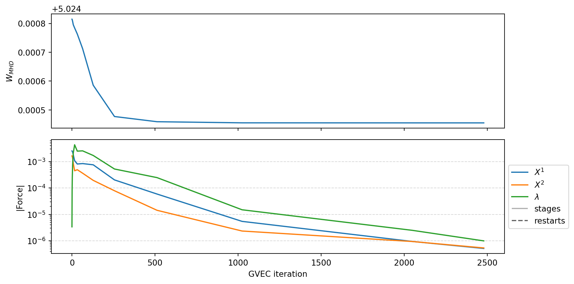
Tokamak: Running GVEC
run = gvec.run(params, runpath="run_tokamak")
GVEC - completed 0/2 stages: |>|.|GVEC - completed 1/2 stages: |=|>|GVEC finished after 0.9 seconds using 2479 iterations (totalIter = 10000) with |force| = 9.97e-07 (minimize_tol = 1.00e-06)
fig = run.plot_diagnostics_minimization()
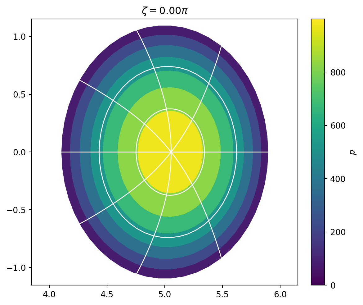
Tokamak: Result
fig, ax = run.state.plot_poloidal_plane("p", zeta=0.0)
Stellarator
- prescribe boundary shape with poloidal & toroidal fourier modes
- prescribe (zero) toroidal current profile
- picard iterations on \(\iota(\rho^2)\)
- minimize MHD energy with fixed rotational transform
Stellarator: Profiles
params = {
"PhiEdge": 1.0,
"iota": {
"type": "polynomial",
"coefs": [0.625, 0.35],
},
"pres": {
"type": "interpolation",
"rho2": [0.0, 0.25, 0.5, 0.75, 1.0],
"vals": [1.0, 0.75, 0.5, 0.25, 0.0],
"scale": 1000.0,
}
}
Stellarator: Profiles
params = {
"PhiEdge": 1.0,
"I_tor": {
"type": "polynomial",
"coefs": [0.0],
},
"picard_current": "auto",
"pres": {
"type": "interpolation",
"rho2": [0.0, 0.25, 0.5, 0.75, 1.0],
"vals": [1.0, 0.75, 0.5, 0.25, 0.0],
"scale": 1000.0,
}
}
Stellarator: Boundary
Boundary represented with double-angle Fourier series:
\[
X^i_b(\vartheta,\zeta) = \sum_{m,n} X^i_{\text{b,cos},m,n} \cos(m\vartheta - n N_{FP} \zeta) + X^i_{\text{b,sin},m,n} \sin(m\vartheta - n N_{FP} \zeta)
\]
Rotating ellipse with three field periods:
\[
\begin{align}
R := X^1_b(\vartheta,\zeta) &= 3.0 + 1.0 \cos\vartheta + 0.4 \cos(\vartheta-3\zeta) \\
Z := X^2_b(\vartheta,\zeta) &= 1.0 \sin\vartheta - 0.4 \sin(\vartheta-3\zeta) - 0.25 \sin(-3\zeta)
\end{align}
\]
params["nfp"] = 1
params["X1_b_cos"] = {
(0, 0): 5.0,
(1, 0): 0.9,
}
params["X2_b_sin"] = {
(1, 0): 1.1,
}
Stellarator: Boundary
Boundary represented with double-angle Fourier series:
\[
X^i_b(\vartheta,\zeta) = \sum_{m,n} X^i_{\text{b,cos},m,n} \cos(m\vartheta - n N_{FP} \zeta) + X^i_{\text{b,sin},m,n} \sin(m\vartheta - n N_{FP} \zeta)
\]
Rotating ellipse with three field periods:
\[
\begin{align}
R := X^1_b(\vartheta,\zeta) &= 3.0 + 1.0 \cos\vartheta + 0.4 \cos(\vartheta-3\zeta) \\
Z := X^2_b(\vartheta,\zeta) &= 1.0 \sin\vartheta - 0.4 \sin(\vartheta-3\zeta) - 0.25 \sin(-3\zeta)
\end{align}
\]
params["nfp"] = 3
params["X1_b_cos"] = {
(0, 0): 3.0,
(1, 0): 1.0,
(1, 1): 0.4,
}
params["X2_b_sin"] = {
(1, 0): 1.0,
(1, 1): -0.4,
(0, 1): -0.25,
}
Stellarator: Numerical Parameters
params["init_average_axis"] = True
params["X1_mn_max"] = [3, 0]
params["X2_mn_max"] = [3, 0]
params["LA_mn_max"] = [3, 0]
params["sgrid"] = {
"nElems": 2
}
params["X1X2_deg"] = 5
params["LA_deg"] = 5
params["totalIter"] = 10000
params["minimize_tol"] = 1e-6
Stellarator: Numerical Parameters
params["init_average_axis"] = True
params["X1_mn_max"] = [3, 3]
params["X2_mn_max"] = [3, 3]
params["LA_mn_max"] = [3, 3]
params["sgrid"] = {
"nElems": 2
}
params["X1X2_deg"] = 5
params["LA_deg"] = 5
params["totalIter"] = 10000
params["minimize_tol"] = 1e-4
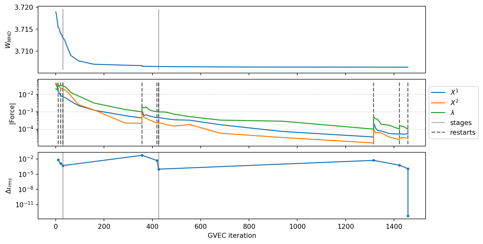
Stellarator: Running GVEC
run = gvec.run(params, runpath="run_stellarator", quiet=True)
state = run.state
fig = run.plot_diagnostics_minimization()
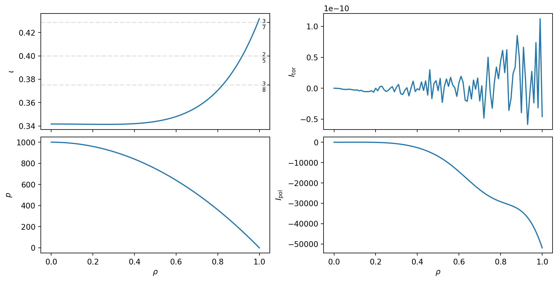
Stellarator: Visualize Profiles
fig, axs = state.plot_radial_profile(["iota", "I_tor", "p", "I_pol"])
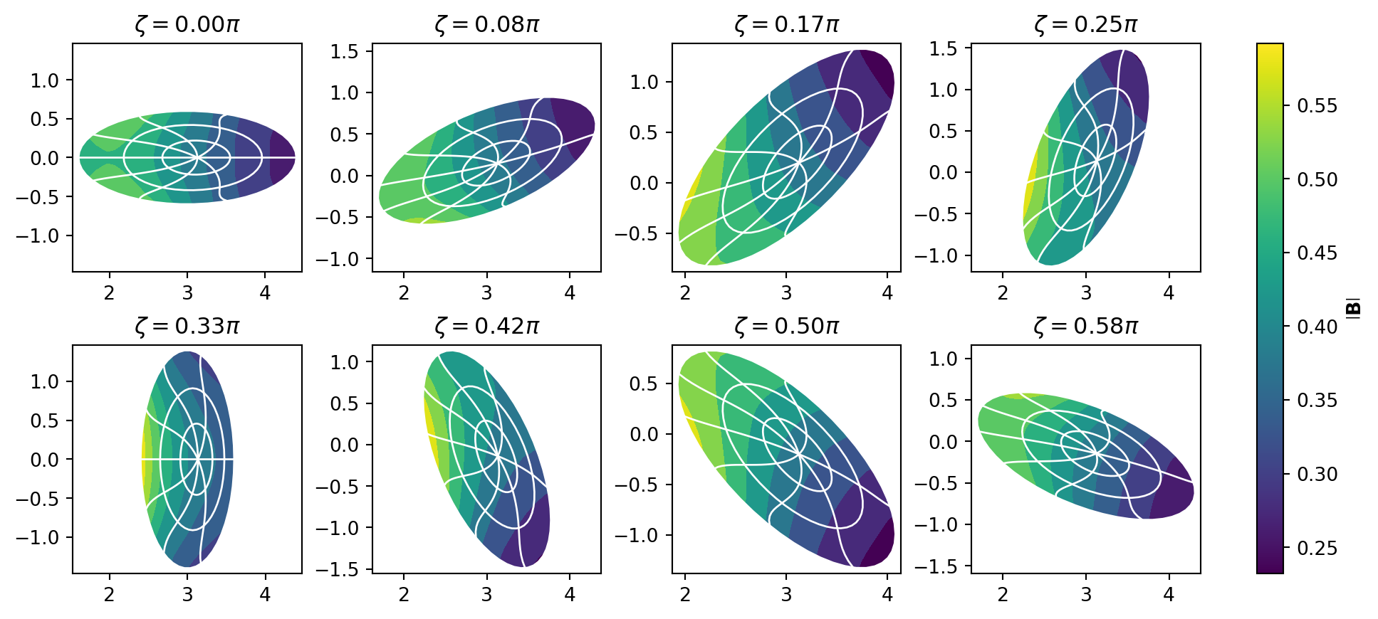
Stellarator: Visualize Cross-sections
fig, axs = state.plot_poloidal_plane(zeta=8, subplot_grid=(2, 4))
Stellarator: 3D Visualization
fig = state.plot_3d_surface("L_gradB", rho=1.0, period="full")
fig.show()
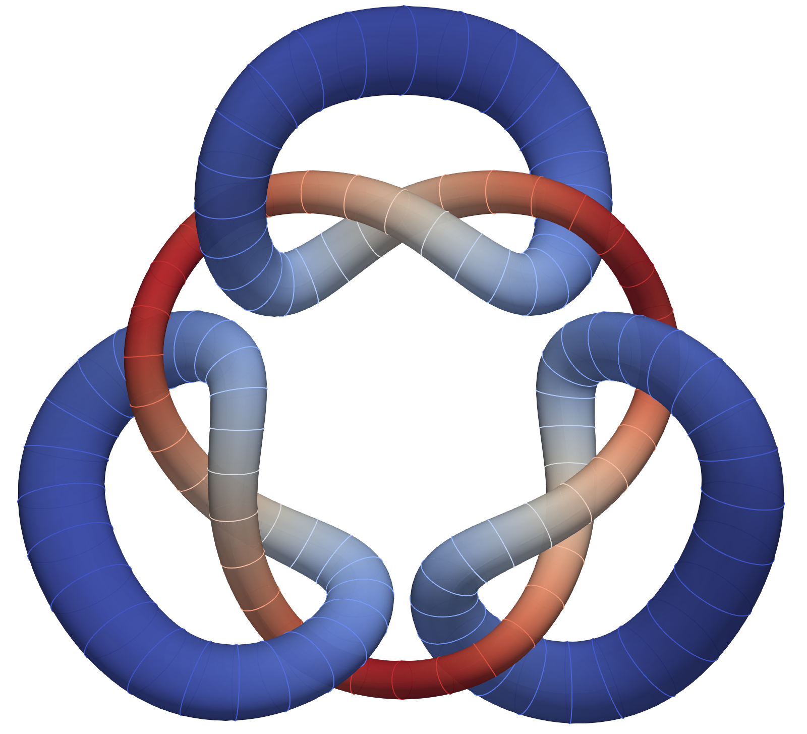
The G-Frame
- Stellarators are not necessarily well represented in cylindrical coordinates
- cross-section not aligned with the plasma
- highly inclined magnetic axis
- straight sections
- knotted axis
- high resolution required, difficult convergence or outright failure
- Solution: align the coordinate frame (toroidal direction) with the plasma
![]()
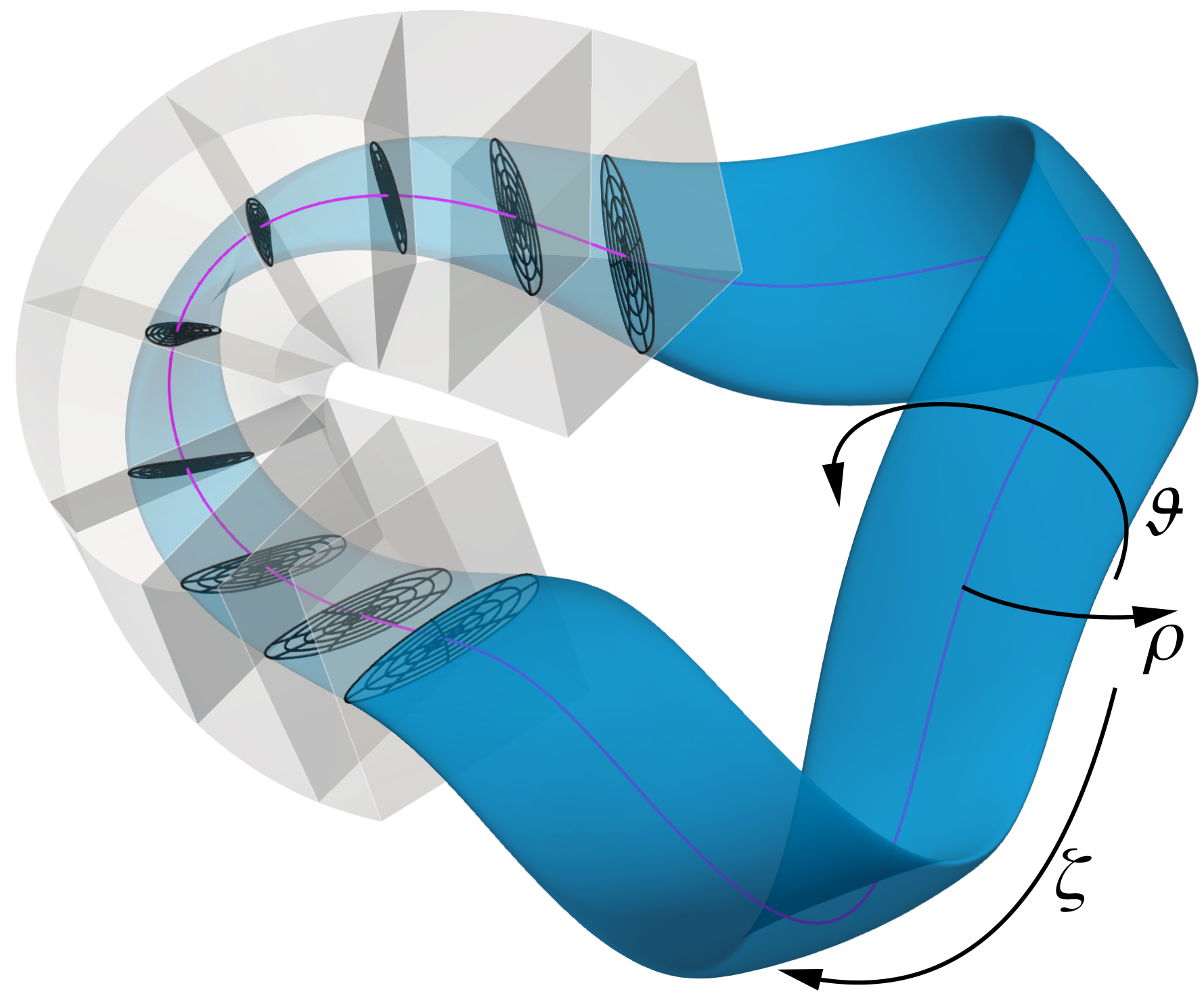
G-Frame
- defined by a guiding curve \(\mathbf{X}_0(\zeta)\)
- planar cross-sections along the curve, defined by \(\mathbf{N}(\zeta), \mathbf{B}(\zeta)\)
- basis vectors \(\mathbf{X}_0', \mathbf{N}, \mathbf{B}\)
- \(f: (\rho,\vartheta,\zeta) \mapsto (q^1,q^2,\zeta) \mapsto (x,y,z)\)
- \(f = g \circ h\)
- find solution \(g: (\rho,\vartheta,\zeta) \mapsto (q^1,q^2,\zeta)\)
- for a fixed \(h: (q^1,q^2,\zeta) \mapsto (x,y,z)\) (cylindrical coordinates or G-Frame)
- constructed from
- a boundary (with “good” parameterization, e.g. Boozer)
- a curve (using a Frenet-Serret frame)
Running GVEC with G-Frame
parameters = dict(
ProjectName="gframe",
which_hmap=21, # G-Frame
hmap_ncfile="../input_surface-Gframe.nc",
getBoundaryFromFile=1,
boundary_filename="../input_surface-Gframe.nc",
X1_mn_max=[3, 4],
X2_mn_max=[3, 4],
LA_mn_max=[3, 4],
X1_sin_cos="_sincos_",
X2_sin_cos="_sincos_",
LA_sin_cos="_sincos_",
X1X2_deg=5,
LA_deg=5,
sgrid=dict(
nElems=5,
),
pres=dict(
type="polynomial",
coefs=[0.0],
),
I_tor=dict(
type="polynomial",
coefs=[0.0],
),
picard_current="auto",
totalIter=10000,
minimize_tol=1e-3,
)
Running GVEC with G-Frame
run = gvec.run(parameters, runpath="run_gframe")
GVEC - completed 0/3 stages, restarts in current stage - 0: |>|.|.|GVEC - completed 1/3 stages, restarts in current stage - 0: |=|>|.|GVEC - completed 2/3 stages, restarts in current stage - 0: |=|=|>|GVEC finished after 3.6 seconds using 206 iterations (totalIter = 10000) with |force| = 9.92e-04 (minimize_tol = 1.00e-03)
and rms Δiota = 8.41e-15(iota_tol=1.00e-03)
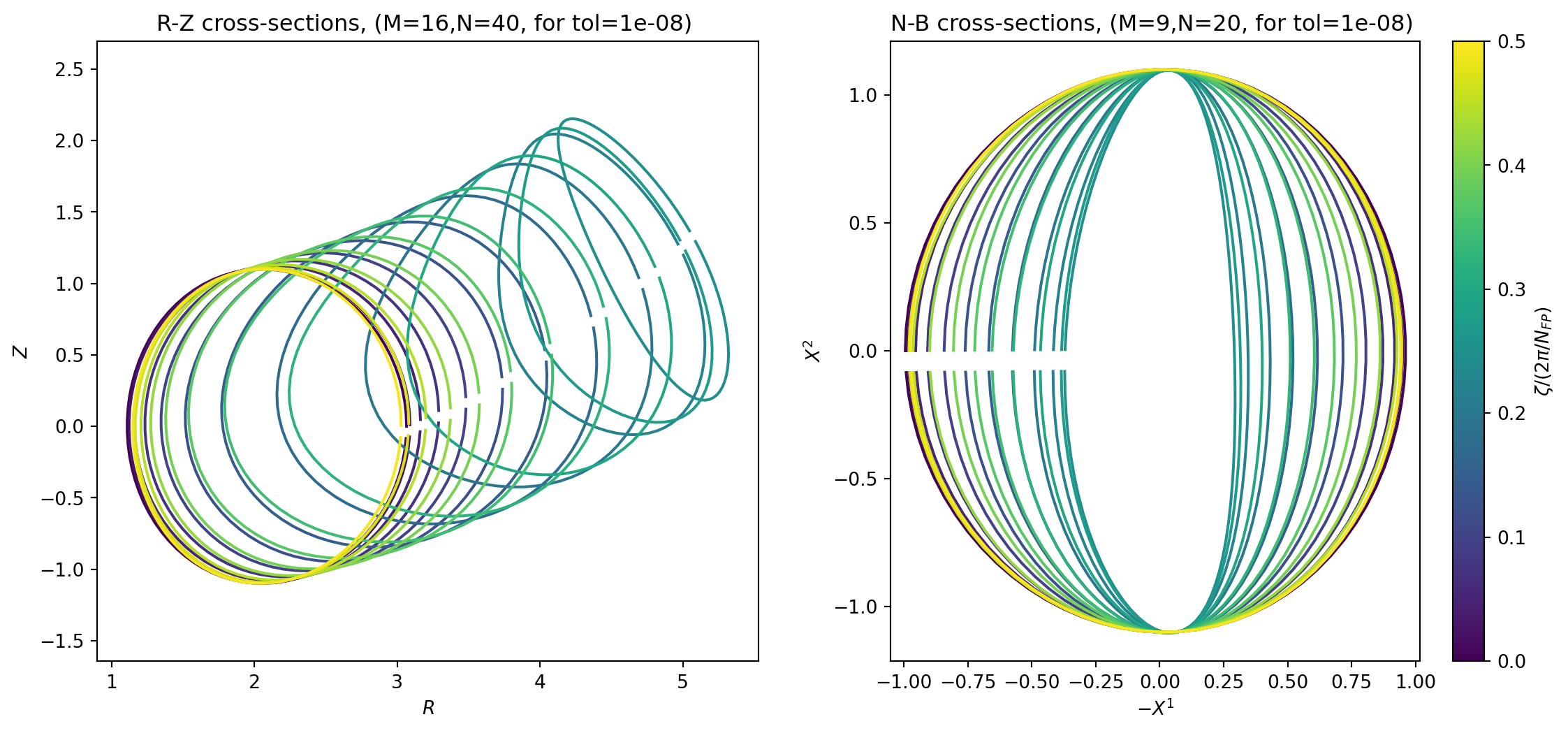
state = run.state
fig, axs = state.plot_poloidal_plane(zeta=8, subplot_grid=(2, 4))
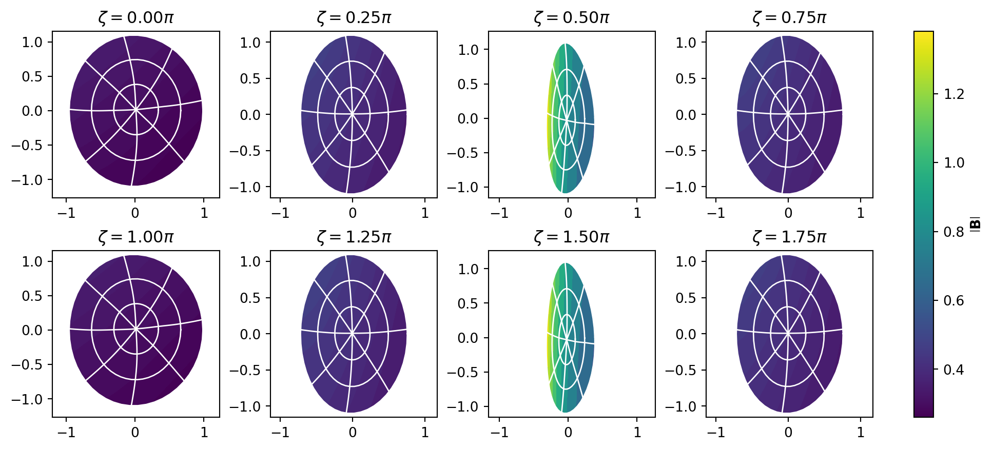
Running GVEC with G-Frame
fig = state.plot_3d_surface("mod_B", rho=1.0, period="full")
fig.show()
More Features
- command line interface:
parameters.toml, pygvec run, pygvec visu …
- more postprocessing & plotting functions
- Boozer & PEST transformation (without projection/interpolation)
- configure multiple stages – e.g. for radial refinement
- fieldline tracing / Poincaré plots for non-cylindrical coordinates
- load boundary & construct G-Frame from a QUASR case
- integration with simsopt (in development)
Thank you for your attention!
![]()
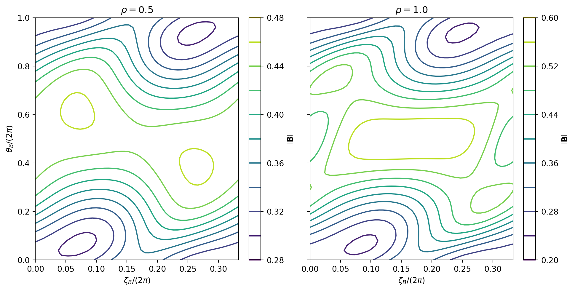
Postprocessing
theta = np.linspace(0, 2 * np.pi, 50)
zeta = np.linspace(0, 2 * np.pi / state.nfp, 8 * 4 + 1)
ev = state.evaluate("pos", "B", rho=[0.5, 1.0], theta=theta, zeta=zeta)
print(ev)
<xarray.Dataset> Size: 1MB
Dimensions: (rad: 2, pol: 50, tor: 33, xyz: 3)
Coordinates:
* rho (rad) float64 16B 0.5 1.0
* theta (pol) float64 400B 0.0 0.1282 0.2565 ... 6.027 6.155 6.283
* zeta (tor) float64 264B 0.0 0.1963 0.3927 0.589 ... 5.89 6.087 6.283
* xyz (xyz) <U1 12B 'x' 'y' 'z'
Dimensions without coordinates: rad, pol, tor
Data variables: (12/44)
X1 (rad, pol, tor) float64 26kB 0.5045 0.4964 ... 0.9758 0.9883
dX1_dr (rad, pol, tor) float64 26kB 0.9732 0.9617 ... 0.9614 0.9681
dX1_dt (rad, pol, tor) float64 26kB 0.008341 0.006512 ... -0.0005496
dX1_dz (rad, pol, tor) float64 26kB 5.451e-15 -0.08317 ... 5.753e-15
dX1_drr (rad, pol, tor) float64 26kB -0.04465 -0.0316 ... 0.02312
dX1_drt (rad, pol, tor) float64 26kB 0.005745 0.004374 ... -0.03973
... ...
Jac (rad, pol, tor) float64 26kB 2.744 2.71 2.529 ... 5.497 5.439
e_theta (xyz, rad, pol, tor) float64 79kB 0.008341 0.006479 ... 1.1
e_zeta (xyz, rad, pol, tor) float64 79kB 1.963e-14 ... -5.255e-15
B_contra_t (rad, pol, tor) float64 26kB 1.001e-16 -0.003144 ... -1.156e-16
B_contra_z (rad, pol, tor) float64 26kB 0.05675 0.05738 ... 0.05264 0.05323
B (rad, pol, tor, xyz) float64 79kB 1.115e-15 ... -4.069e-16
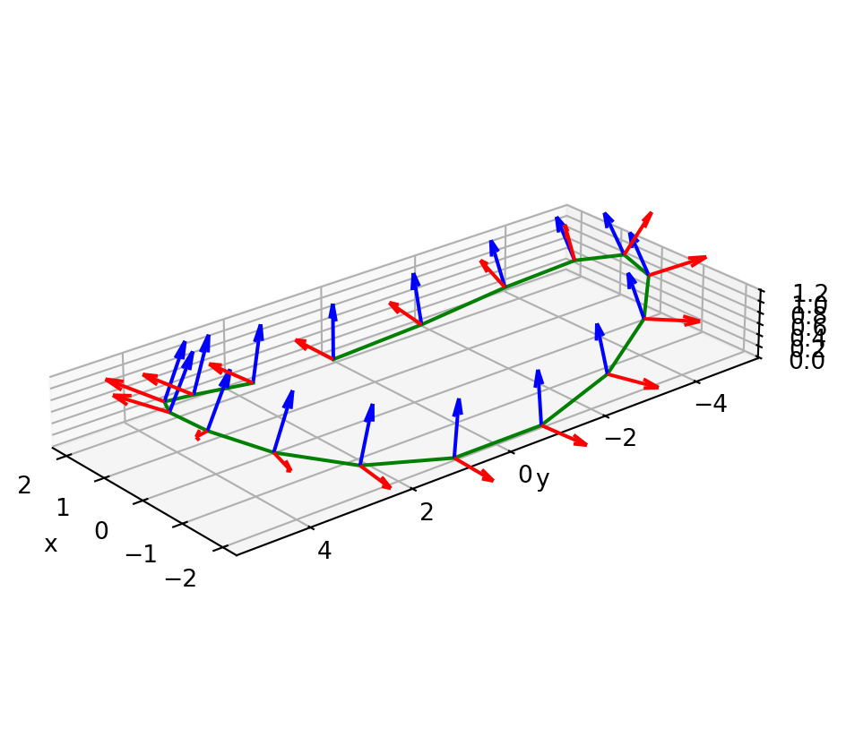
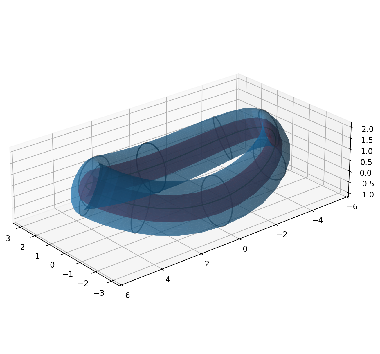
Postprocessing
fig = plt.figure(figsize=(8, 8))
ax = fig.add_subplot(111, projection="3d", alpha=0.9)
# last surface in rho
ax.plot_surface(*ev.pos.sel(rho=1.0, method="nearest"), alpha=0.5)
# cuts of the boundary
for t in range(0, ev.tor.size, 4):
ax.plot3D(
*ev.pos.isel(rad=-1, tor=t), alpha=0.5, color="k"
)
# flux surface mid-radius
ax.plot_surface(*ev.pos.sel(rho=0.5, method="nearest"), alpha=0.5, color="red")
ev_axis = state.evaluate("pos", rho=0.0, theta=0.0, zeta=np.linspace(0, 2 * np.pi, 201))
ax.plot3D(*ev_axis.pos, color="green")
ax.set(aspect="equal")
ax.view_init(25, 140, 0)
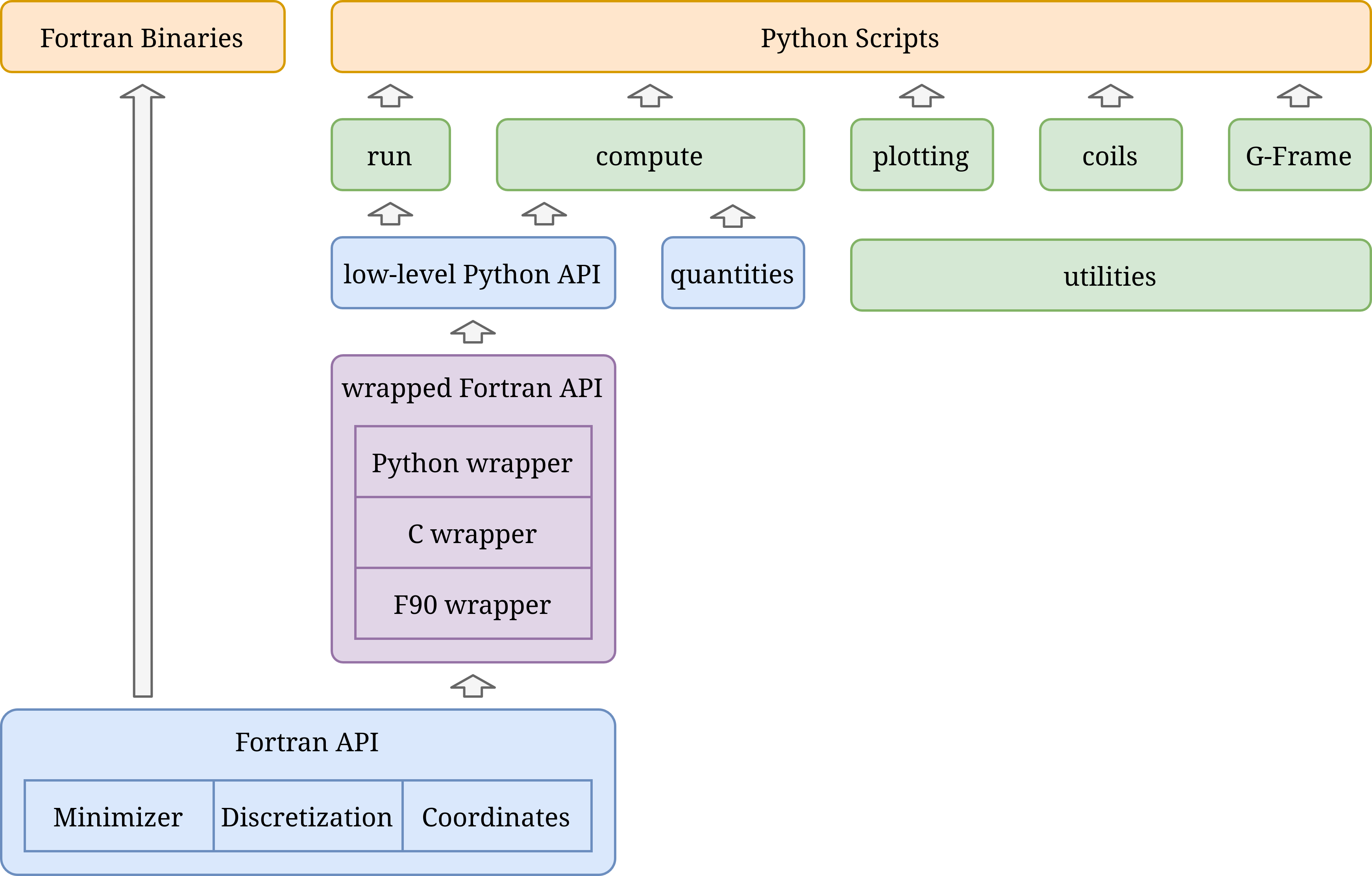
Structure
![]()
Software Stack
- Build system:
CMake & scikit-build-core (using Find_Package & PkgConfig)
- Python – Fortran:
f90wrap & numpy-f2py
- Fortran:
SeLaLib, BLAS, ftimings, OpenMP, MPI
- Python:
xarray, numpy, scipy, matplotlib, plotly, …
Quantities
- \(X^1, X^2, \lambda, \pqdx{X^1}{\rho}, \pqdxy{X^2}{\vartheta}{\zeta}, \dots\)
- \(\mathcal{J}, \vec{e}_\rho, \grad_\rho, g_{\vartheta\zeta}, \vec{k}_{\vartheta\zeta}, II_{\vartheta\zeta}, \dots\)
- \(\iota, p, \Phi, \chi, \dqdx{\iota}{\rho}, \dqdxx{p}{\rho}, \dots\)
- \(\vec{B}, \vec{J}, \vec{F}, B^\vartheta, \overline{B_\zeta}, \dots\)
- \(\vartheta_P, B^{\vartheta_P}, g_{\vartheta_P\zeta_P}, \dots\)
- \(\nu_B, \pqdx{\nu_B}{\rho}, B^{\vartheta_B}, g_{\vartheta_B\zeta_B}, \dots\)
- \(I_\text{tor}, \Delta_\text{mirror}, \beta_\text{avg}, L_{\grad\vec{B}}, \kappa_G, \dots\)
@register(
requirements=("p", "mod_B", "Jac", "V", "mu0"),
integration=("rho", "theta", "zeta"),
attrs=dict(
long_name="volume-averaged plasma beta",
symbol=r"\overline{\beta}",
),
)
def beta_avg(ds: xr.Dataset):
beta = 2 * ds.mu0 * ds.p / ds.mod_B**2
ds["beta_avg"] = volume_integral(beta * ds.Jac) / ds.V
Constructing a G-Frame from a boundary
xyz = np.load("input_surface.npy") # shape (n_zeta, n_theta, 3)
Constructing a G-Frame
parameters_constructed, gframe_constructed = (
gvec.gframe.construct_gframe_from_surface(
xyz,
nfp=2,
name="surface_constructed",
tolerance_output=1e-3,
cutoff_gframe=8,
)
)
- fit planes to \(\zeta\)-contours
- construct \(\mathbf{X}_0(\zeta),\mathbf{N}(\zeta),\mathbf{B}(\zeta)\) as fourier series with
cutoff_gframe modes
- can enforce field periodicity & stellarator symmetry
- cut input surface with the planes: get \(X^1(\vartheta,\zeta), X^2(\vartheta,\zeta)\)
- can enforce stellarator symmetry
- find minimal mode numbers \(m,n\) for \(X^1, X^2\) with max distance
tolerance_output
- write G-Frame file (frame & boundary) & parameter file
Constructing a G-Frame
surface_constructed = gvec.gframe.to_surface(gframe_constructed, nzeta=20)
Constructing a G-Frame
for key, value in parameters_constructed.items():
print(f"{key:20}: {value}")
ProjectName : surface_constructed
which_hmap : 21
hmap_ncfile : surface_constructed-Gframe.nc
X1X2_deg : 5
LA_deg : 5
sgrid : {'grid_type': 0, 'nElems': 5}
X1_mn_max : (3, 4)
X2_mn_max : (3, 4)
LA_mn_max : (3, 4)
X1_sin_cos : _sincos_
X2_sin_cos : _sincos_
LA_sin_cos : _sincos_
minimize_tol : 1e-07
totalIter : 100000
logIter : 100
pres : {'type': 'polynomial', 'coefs': [0.0]}
I_tor : {'type': 'polynomial', 'coefs': [0.0]}
picard_current : auto
getBoundaryFromFile : 1
boundary_filename : surface_constructed-Gframe.nc
Constructing a G-Frame
parameters_constructed["hmap_ncfile"] = "../" + parameters_constructed["hmap_ncfile"]
parameters_constructed["boundary_filename"] = "../" + parameters_constructed["boundary_filename"]
parameters_constructed["minimize_tol"] = 1e-3
runpath = "run_constructed_gframe"
run = gvec.run(parameters_constructed, runpath=runpath)
GVEC - completed 0/3 stages, restarts in current stage - 0: |>|.|.|GVEC - completed 1/3 stages, restarts in current stage - 0: |=|>|.|GVEC - completed 2/3 stages, restarts in current stage - 0: |=|=|>|GVEC finished after 3.1 seconds using 157 iterations (totalIter = 100000) with |force| = 9.87e-04 (minimize_tol = 1.00e-03)
and rms Δiota = 2.72e-14(iota_tol=1.00e-03)